10 Best Google Sheets Budget Templates & Free Trackers (2026)

Most people open a blank spreadsheet to start budgeting, stare at the empty grid for five minutes, and close the tab. A good budget template gives you the structure, formulas, and categories already built so you can start tracking your money in the next ten minutes instead of the next week.

This guide covers the best free Google Sheets and Excel budget templates available in June 2026, walks you through building a custom budget dashboard from scratch, and shows you how to set up a real-time inventory tracker without paying for software. You'll get the exact formulas, column structures, and decision frameworks to choose between free templates and paid bundles.

Best Free Google Sheets Budget Templates for 2026

Free budget templates fall into three proven frameworks: zero-based (assign every dollar a job), envelope (allocate cash to spending categories), and 50/30/20 (split income into needs, wants, and savings). The best templates in June 2026 automate the math, include visual progress tracking, and let you customize categories without breaking formulas.

Aspire Budgeting: Zero-Based Envelope System

Aspire Budgeting remains the most complete free Google Sheets budget option because it implements zero-based envelope budgeting with running balances, rollover logic, and monthly reconciliation built in. Most budget templates give you a grid to fill in numbers, but they don't help you actually manage your money over time.

The setup takes about 20 minutes. You create one row per spending envelope (groceries, rent, gas, dining out), enter your income, and assign every dollar to an envelope before the month starts. As you spend, you log transactions in the Transactions tab, and the template automatically deducts from the correct envelope balance. If you overspend in one category, you see it immediately and can move money from another envelope to cover it.

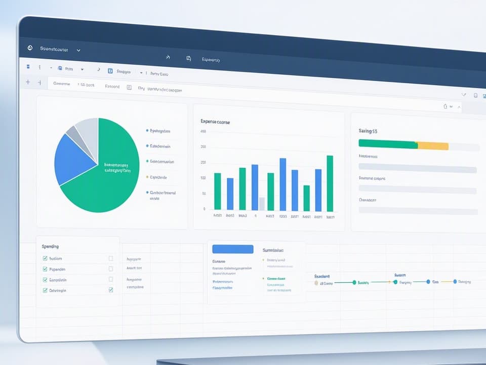
The template includes a dashboard tab that shows your total unassigned cash, spending by category, and progress toward savings goals. You can duplicate the template for each month or use the built-in archive feature to compare spending year-over-year. The formulas are visible and well-commented, so if you want to add a custom category or change the rollover logic, you can do it without breaking the entire sheet.

Aspire works best for people who want hands-on control and don't mind logging every transaction manually. If you prefer to link your bank account and auto-import transactions, you'll need a paid app like Tiller or YNAB instead.

Google Sheets Native Monthly and Annual Budget Templates

Google's built-in Monthly Budget and Annual Budget templates are surprisingly capable for most people who just want to track income, expenses, and savings without learning a budgeting methodology. Both templates include auto-calculated totals, pre-built category lists, and simple bar charts that update as you enter data.

To access them, open Google Sheets, click Template Gallery at the top, and select Monthly Budget or Annual Budget under Personal. The Monthly Budget template gives you a single-month view with income at the top, fixed expenses in the middle, and variable expenses below. The Annual Budget template spreads twelve months across columns so you can see seasonal patterns and compare spending month-to-month.

Both templates use basic SUM formulas and conditional formatting to highlight overspending. If your actual expenses exceed your budgeted amount in any category, the cell turns red. The charts auto-update, so you get a visual breakdown of spending by category without building pivot tables or custom graphs.

Customization is straightforward. Add rows for new categories, copy formulas down, and adjust the chart data range if needed. The templates don't include envelope logic or transaction logs, so they work best if you review bank statements weekly and enter totals by category rather than logging every purchase.

50/30/20 Budget Template Options

The 50/30/20 framework splits your after-tax income into three buckets: 50% for needs (rent, utilities, groceries), 30% for wants (dining out, subscriptions, hobbies), and 20% for savings and debt repayment. Free templates that implement this split calculate the target amounts for each bucket automatically and show you how much room you have left in each category.

A solid 50/30/20 template includes three sections. The top section calculates your monthly take-home income and multiplies it by 0.5, 0.3, and 0.2 to show your target spending in each bucket. The middle section lists your actual expenses with a dropdown or manual tag for needs, wants, or savings. The bottom section uses SUMIF formulas to total spending by category and compare it to your targets.

The formula breakdown looks like this: =SUMIF(B:B,"Needs",C:C) sums all amounts in column C where column B equals "Needs". You repeat this for wants and savings, then subtract actual from target to see how much budget remains. Conditional formatting turns the remaining balance red when you exceed the target.

These templates work well for people who want a simple rule to follow without tracking every spending category separately. The downside is that the 50/30/20 split is a rough guideline, not a personalized budget. If your rent eats 40% of your income, you'll need to adjust the percentages or switch to a zero-based approach.

When to Use a Pre-Built Budget Template vs. Building Your Own

Use a pre-built template if you're starting from zero, need to track spending this week, or want a proven framework like envelope budgeting without researching the methodology first. Build your own if you have specific tracking needs (multiple income streams, irregular expenses, shared household budgets), want full control over formulas, or enjoy spreadsheet customization.

For most people, the Google Sheets Monthly Budget template or Microsoft Excel's Personal Monthly Budget template is more than enough. Both are free, easy to customize, and built by the platform owners so they stay updated. Start with a template, use it for two months, and then decide if you need more features or want to rebuild it from scratch.

The decision point is time investment versus customization. A pre-built template gets you tracking in 10 minutes but might not fit your exact workflow. Building your own takes 2-3 hours but gives you exactly the categories, formulas, and dashboard layout you want. If you're not sure, start with a template and migrate later.

How to Build a Budget Dashboard in Excel from Scratch

A budget dashboard pulls data from multiple input sheets (income, expenses, savings goals) and displays it in one visual summary with charts, progress bars, and key metrics. Building one from scratch in Excel takes about two hours and gives you full control over layout, formulas, and chart types.

The core structure uses three sheets: Data (raw transactions), Summary (category totals), and Dashboard (visual display). The Data sheet holds every income and expense entry with columns for date, category, amount, and description. The Summary sheet uses pivot tables or SUMIF formulas to calculate totals by category and month. The Dashboard sheet links to the Summary sheet and displays charts, conditional formatting, and progress bars.

Setting Up Your Data Tables and Input Sheets

Start with the Data sheet. Create five columns: Date (formatted as date), Category (dropdown list), Amount (currency), Type (Income or Expense dropdown), and Description (text). Use Data Validation to create dropdown lists for Category and Type so you don't end up with typos like "Grocerys" and "Grocery" that break your formulas.

To create the Category dropdown, list all your categories in a separate reference sheet (Rent, Utilities, Groceries, Dining Out, Transportation, Entertainment, Savings). Then select the Category column in your Data sheet, go to Data > Data Validation, choose List from a range, and point it to your category list. Repeat for the Type column with just two options: Income and Expense.

Add a header row and freeze it so column names stay visible as you scroll. Format the Date column as Short Date, the Amount column as Currency, and apply alternating row colors for readability. This setup lets you log transactions quickly without worrying about formula errors from inconsistent category names.

Creating Dynamic Charts and Pivot Tables

Pivot tables summarize your transaction data by category, month, or type without writing complex formulas. To create one, select your entire Data range including headers, go to Insert > PivotTable, and place it on a new sheet called Summary. Drag Category to Rows, Amount to Values, and Type to Filters. Set the filter to show only Expense, and you'll see total spending by category.

For a monthly breakdown, add Date to Columns and group it by month. Right-click any date in the pivot table, choose Group, and select Months. Now you have a grid showing spending by category across months, which updates automatically when you add new transactions to the Data sheet.

Charts work best when they answer a specific question. A pie chart shows spending breakdown by category. A column chart compares monthly spending over time. A line chart tracks savings balance month-to-month. To create a chart, select the pivot table data you want to visualize, go to Insert > Charts, and choose the type that fits your question.

Link the charts to your Dashboard sheet by copying them (Ctrl+C) and pasting them as linked pictures (Paste Special > Linked Picture). This keeps the Dashboard clean and ensures charts update when the underlying data changes.

Adding Conditional Formatting and Progress Bars

Conditional formatting highlights overspending, tracks progress toward goals, and adds visual cues without cluttering your dashboard with text. The most useful rules are color scales (green for under budget, red for over) and data bars (horizontal bars that fill based on percentage of goal).

To add a color scale, select the cells showing budget vs. actual spending, go to Home > Conditional Formatting > Color Scales, and choose a three-color scale (green, yellow, red). Excel automatically applies the gradient based on cell values, so categories where you're under budget appear green and overspending appears red.

Data bars work well for savings goals and spending limits. If you're saving for a $5,000 emergency fund and have $3,200 saved, a data bar fills 64% of the cell width. To add one, select the cell showing current savings, go to Conditional Formatting > Data Bars, and choose a solid fill color. Adjust the bar's maximum value to match your goal so the bar fills completely when you hit the target.

For more control, use custom formulas with conditional formatting. If you want to highlight any category where actual spending exceeds budget by more than 10%, select the actual spending column, choose Conditional Formatting > New Rule > Use a formula, and enter =B2>C2*1.1 (assuming column B is actual and column C is budget). Format the cell with a red fill, and Excel applies it only when the condition is true.

Linking Multiple Sheets for a Unified Dashboard View

The Dashboard sheet pulls data from the Summary sheet using cell references and formulas. Instead of copying and pasting values (which break when the source data updates), link directly to the cells you want to display.

To link a cell, type = in the Dashboard sheet, switch to the Summary sheet, click the cell you want to reference, and press Enter. Excel creates a formula like =Summary!B5 that updates automatically. For entire ranges, use formulas like =Summary!B5:B15 or reference named ranges for cleaner formulas.

Named ranges make dashboard formulas easier to read and maintain. If your total monthly spending is in cell Summary!D10, select that cell, go to Formulas > Define Name, and name it TotalSpending. Now you can use =TotalSpending in your dashboard instead of =Summary!D10, and if you move the cell later, the formula still works.

Use INDIRECT if you want to dynamically change which month or category the dashboard displays. Create a dropdown in cell A1 with month names, then use =INDIRECT("Summary!"&A1&"!B5") to pull data from the sheet named after the selected month. This technique lets you build a dashboard that switches between months without manually updating formulas.

Free Google Sheets Inventory Tracker Setup Guide

Google Sheets is a viable, free option for inventory tracking, especially for small businesses or teams getting started with structured stock management. Its real-time collaboration features make it easy for multiple team members to update inventory data simultaneously without version conflicts or email attachments.

An inventory tracker needs six core functions: record current stock levels, flag low-stock items, calculate total inventory value, log stock movements (in and out), track supplier information, and provide an audit trail. You can build all six in Google Sheets using basic formulas, conditional formatting, and sharing settings.

Essential Columns for Inventory Tracking

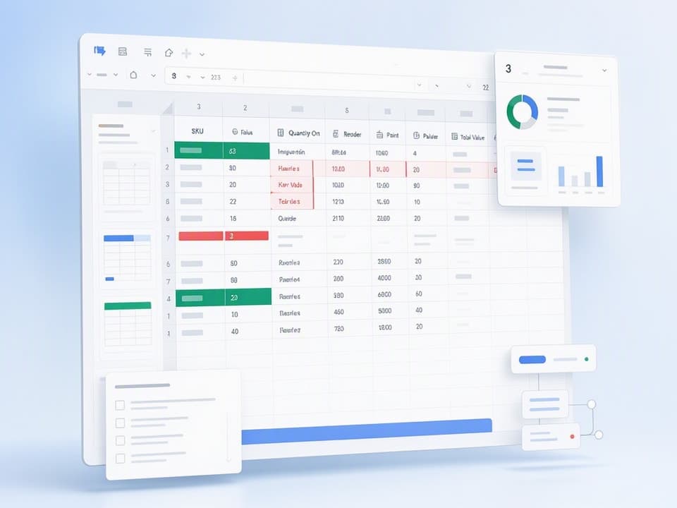
Start with a single sheet called Inventory. Create eight columns: SKU (unique product code), Product Name, Category (dropdown for product type), Quantity on Hand, Reorder Point, Unit Cost, Total Value, Supplier, and Last Updated. The SKU column ensures each product has a unique identifier even if names are similar.

Format Quantity on Hand and Reorder Point as numbers with no decimals. Format Unit Cost and Total Value as currency. Use Data Validation to create a dropdown for Category so all team members use consistent labels (Raw Materials, Finished Goods, Packaging, Supplies). Add a Last Updated column formatted as date and time, and use =NOW() to automatically timestamp when a row is edited.

The Total Value column uses a simple formula: =D2*F2 (Quantity on Hand times Unit Cost). Copy this formula down for every product. At the bottom of the Total Value column, use =SUM(G2:G100) to calculate total inventory value across all items. This number helps you track carrying costs and insurance requirements.

Add a Notes column if you need to track batch numbers, expiration dates, or location within a warehouse. Keep the core columns consistent across all rows so you can use filters and pivot tables to analyze inventory by category or supplier.

Formulas for Automatic Reorder Alerts and Stock Valuation

Reorder alerts prevent stockouts by flagging items that fall below a safe threshold. Use conditional formatting to highlight rows where Quantity on Hand is less than or equal to Reorder Point. Select the Quantity on Hand column, go to Format > Conditional formatting, choose "Less than or equal to", and reference the Reorder Point column. Set the format to a red fill or bold red text.

For a more visible alert, add a Status column with a formula: =IF(D2<=E2,"REORDER","OK"). This creates a text flag you can filter on to see all items that need reordering. Combine it with conditional formatting to color-code the status (red for REORDER, green for OK).

Stock valuation uses SUMIF to calculate inventory value by category or supplier. If you want to know the total value of Finished Goods inventory, use =SUMIF(C:C,"Finished Goods",G:G) where column C is Category and column G is Total Value. Repeat this formula for each category to build a summary table.

For inventory turnover, add a Sales or Usage column that tracks how many units you sold or used in the last month. Calculate turnover as =Sales/Average Inventory. A turnover ratio above 4 means you're moving inventory quickly; below 2 suggests overstocking. This metric helps you decide when to reduce order quantities or clear slow-moving items.

Enabling Real-Time Collaboration and Mobile Access

Real-time collaboration is Google Sheets' biggest advantage over Excel for inventory tracking. Click Share in the top right, add team members by email, and set permissions to Editor so they can update stock levels. Changes appear instantly for everyone viewing the sheet, and Google Sheets tracks who made each edit in the version history.

To prevent accidental formula deletion, protect the formula cells. Select the Total Value column (which contains formulas), right-click, choose Protect range, and set permissions so only you can edit those cells. Team members can still update Quantity on Hand and other input columns, but they can't break the formulas that calculate totals.

For mobile access, install the Google Sheets app on iOS or Android. The app lets you scan barcodes (if your SKUs are barcode-compatible), update quantities, and view the full inventory tracker from a warehouse floor or retail location. Use the filter feature to quickly find a specific SKU or product name without scrolling through hundreds of rows.

Version history provides an audit trail for inventory changes. Go to File > Version history > See version history to view every edit with timestamps and user names. If someone accidentally deletes a row or changes a quantity incorrectly, you can restore a previous version or see exactly what changed and when.

When Carrying Costs Justify a Paid Inventory System

Carrying costs for inventory average 20-30% of total inventory value annually, covering storage, insurance, obsolescence, and opportunity cost. If your inventory value exceeds $50,000, you're spending $10,000-$15,000 per year just to hold that stock. At this scale, a paid inventory system that reduces stockouts, speeds up reordering, or improves turnover can pay for itself in saved carrying costs.

Google Sheets works well up to about 500 SKUs and 5 users. Beyond that, performance slows, collaboration becomes harder to manage, and the risk of data errors increases. If you're spending more than 5 hours per week maintaining your inventory spreadsheet, it's time to evaluate paid options like Sortly, Zoho Inventory, or Fishbowl.

The decision point is when manual tracking costs more than software. If your team spends 10 hours per week on inventory updates, reconciliation, and reporting, that's $5,000-$10,000 per year in labor at $25-$50 per hour. A paid system at $100-$300 per month ($1,200-$3,600 per year) saves money and reduces errors.

Start with Google Sheets to prove the workflow and understand your tracking needs. After six months, if you're hitting the limits of spreadsheet-based tracking, you'll know exactly which features you need in a paid system and can choose one that fits your workflow instead of adapting your workflow to the software.

Microsoft Excel's Built-In Budget and Inventory Templates

Microsoft Excel offers free built-in budget templates for personal, family, and event budgeting, plus inventory templates for small business stock tracking. These templates are professionally designed, formula-ready, and available in Excel for Windows, Mac, and Excel Online without a Microsoft 365 subscription.

To access them, open Excel, click New, and browse the template gallery. Type "budget" or "inventory" in the search bar to filter results. Each template includes a preview screenshot, description, and download button. Once downloaded, the template opens as a new workbook you can customize and save.

Personal and Family Budget Templates in Excel

Excel's Personal Monthly Budget template is the closest equivalent to Google Sheets' Monthly Budget. It includes sections for income, housing, transportation, food, and savings, with auto-calculated totals and a summary chart. The template uses simple SUM formulas and percentage calculations to show how much of your income goes to each category.

The Family Budget Planner template adds shared expense tracking and multiple income sources, useful for households with two earners or roommates splitting costs. It includes a tab for each month and a summary tab that rolls up the year. The formulas link across tabs, so entering data in January automatically updates the annual summary.

Excel's advantage over Google Sheets is offline access and faster performance with large data sets. If you track thousands of transactions or build complex dashboards with multiple pivot tables, Excel handles it better than Google Sheets. The downside is that collaboration requires OneDrive and Excel Online, which don't support all desktop Excel features.

For most people, the choice between Excel and Google Sheets comes down to ecosystem preference. If you already use Microsoft 365 for work and store files in OneDrive, Excel templates integrate seamlessly. If you use Google Workspace or prefer browser-based tools, Google Sheets templates are the better fit.

Excel Inventory Templates for Small Business

Excel's Inventory List template includes columns for SKU, product name, quantity, reorder level, and supplier information, similar to the Google Sheets setup described earlier. The template uses conditional formatting to highlight low-stock items and includes a summary section showing total inventory value and items below reorder point.

The Business Inventory template adds purchase order tracking, received quantities, and sold quantities, giving you a full stock movement history. This template works well for retail stores or small manufacturers who need to track inventory in, out, and on hand. The formulas automatically calculate current stock as starting inventory plus received minus sold.

Excel's inventory templates are downloadable from the template gallery at excel.cloud.microsoft. The templates are free and don't require a Microsoft 365 subscription, but you need Excel installed on your computer or access to Excel Online to use them.

For businesses that need barcode scanning, multi-location tracking, or integration with accounting software, Excel's built-in templates hit their limits quickly. Use them to start, then migrate to a dedicated inventory system like QuickBooks, Zoho Inventory, or Cin7 when you outgrow spreadsheet-based tracking.

Recommended Resources

Skip the blank-sheet setup

Start with the dashboard structure already built so you can track budgets and inventory in minutes, not hours

TemplateGoogle Sheets, Excel.

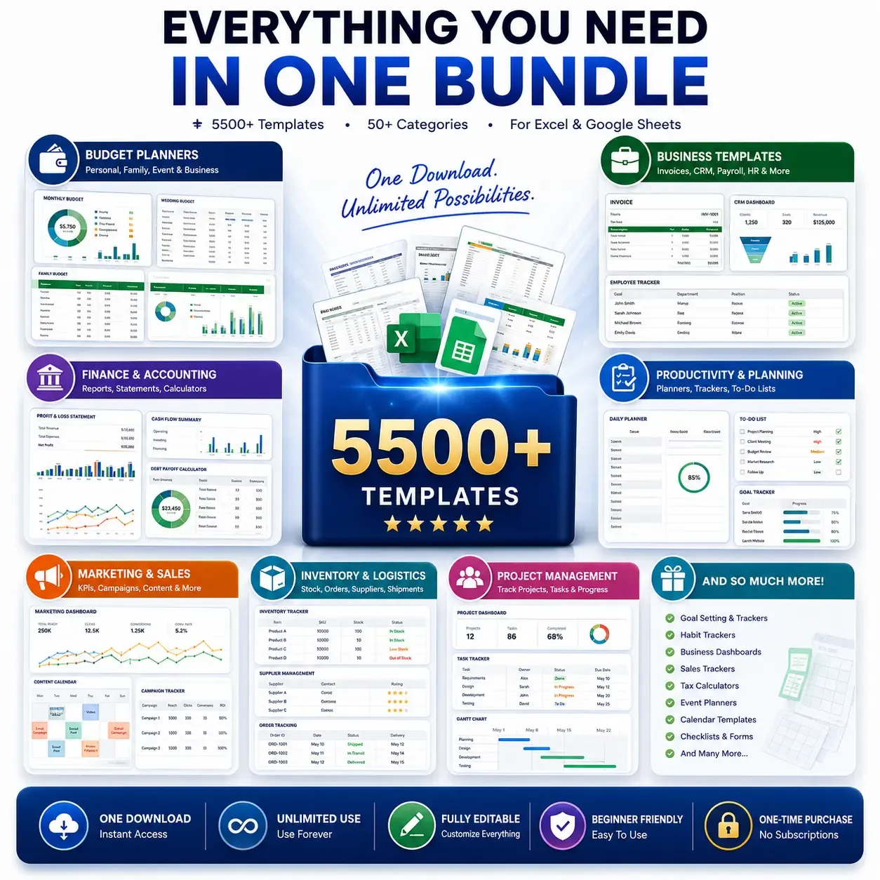
5500+ Ms Excel Templates Mega Bundle – Google Sheet Supported

Learn moreView product

TemplateGoogle Sheets, Excel.

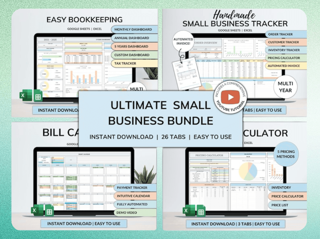
Ultimate Small Business Bundle Templates - Google Sheet + Ms Excel

All-in-One Spreadsheets for Bookkeeping, Inventory, Orders, Billing & Pricing Save Hours Every Week: Automate data entry and dashboards so you can focus on growth, not spreadsheets.

View product

TemplateGoogle Sheets, Excel.

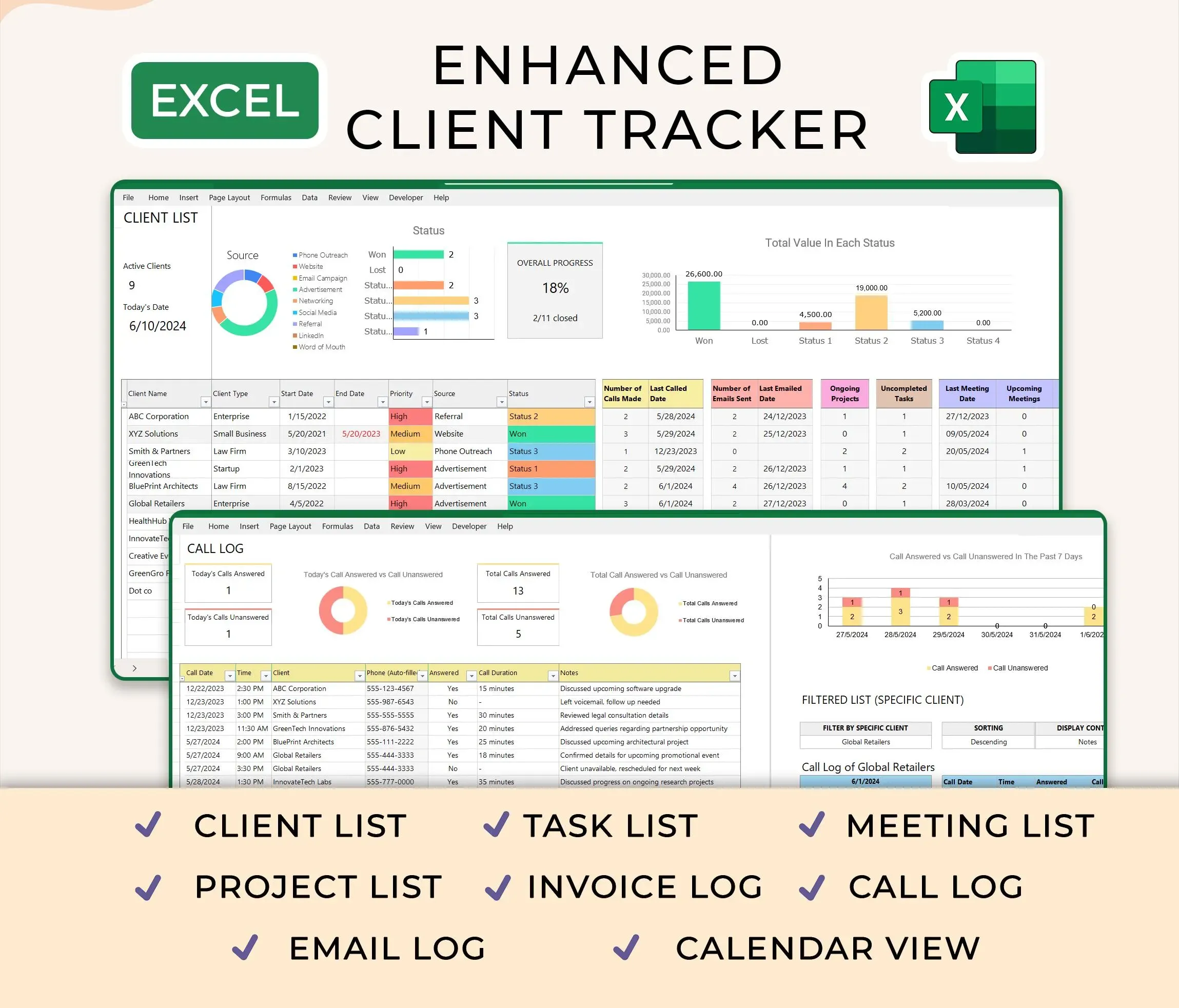
Ultimate Client Tracker CRM Template – Google Sheet & Ms Excel Versions

Learn moreView product

Advanced Budgeting Methodologies in Spreadsheets

Zero-based, envelope, and priority-based budgeting are the three most effective methodologies for spreadsheet users who want more control than a simple income-minus-expenses tracker. Each methodology solves a different problem: zero-based prevents unallocated money from disappearing, envelope stops overspending in any category, and priority-based adapts to variable income.

You can implement all three in Google Sheets or Excel using basic formulas, but the setup differs for each. Zero-based requires monthly resets and allocation tracking. Envelope needs running balances and rollover logic. Priority-based uses tiered spending categories and flexible allocation rules.

Zero-Based Budgeting: Assigning Every Dollar a Job

Zero-based budgeting means your income minus all budget allocations equals zero at the start of each month. Every dollar has an assigned purpose (rent, groceries, savings, debt repayment) before you spend anything. This prevents lifestyle creep and forces you to prioritize spending.

The formula setup uses three columns: Category, Budgeted Amount, and Remaining to Allocate. At the top of the sheet, enter your total monthly income. Below that, list every spending category and assign a dollar amount to each. At the bottom, use =Income - SUM(Budgeted Amounts) to calculate unallocated money. The goal is to get this number to zero.

As the month progresses, log actual expenses in a separate Transactions sheet. Use SUMIF to calculate actual spending by category: =SUMIF(Transactions!B:B,"Groceries",Transactions!C:C). Compare actual to budgeted to see if you're on track. If you overspend in one category, reduce the budget in another to keep total allocations equal to income.

Monthly reconciliation is critical. At the end of the month, check if any categories have money left over. Roll it into next month's budget, move it to savings, or reallocate it to a category where you overspent. Then reset all actual spending to zero and start the new month with a fresh budget.

Envelope Budgeting in Digital Spreadsheets

Envelope budgeting allocates cash to spending categories (envelopes) at the start of the month, and you can only spend what's in each envelope. When an envelope is empty, you stop spending in that category or transfer money from another envelope. The digital version uses spreadsheet formulas to track envelope balances instead of physical cash.

Create three sheets: Envelopes, Transactions, and Dashboard. The Envelopes sheet lists each spending category with columns for Starting Balance, Spent This Month, and Current Balance. The formula for Current Balance is =Starting Balance - Spent This Month. Starting Balance equals last month's ending balance plus this month's new allocation.

The Transactions sheet logs every purchase with columns for Date, Category, Amount, and Envelope. Use Data Validation to create a dropdown for Envelope that matches your envelope names exactly. In the Envelopes sheet, use SUMIF to calculate Spent This Month: =SUMIF(Transactions!D:D,"Groceries",Transactions!C:C).

Rollover logic is what makes envelope budgeting work. If you budget $400 for groceries but only spend $350, the remaining $50 rolls into next month's starting balance. If you overspend by $30, next month starts with a $30 deficit. This creates a natural incentive to stay within limits because overspending today means less money available tomorrow.

The Dashboard sheet shows all envelope balances in one view, with conditional formatting to highlight negative balances (overspending) in red. Add a chart showing envelope balances over time to spot trends and adjust allocations.

Priority-Based Budgeting for Variable Income

Priority-based budgeting works for freelancers, gig workers, and anyone with irregular income. Instead of budgeting a fixed amount per category, you rank expenses by priority (must-pay, important, nice-to-have) and allocate income to higher-priority categories first.

Create four priority tiers: Tier 1 (rent, utilities, minimum debt payments), Tier 2 (groceries, transportation, insurance), Tier 3 (savings, extra debt payments, subscriptions), and Tier 4 (dining out, entertainment, hobbies). List all expenses under the appropriate tier and sum each tier's total.

When income arrives, allocate it to Tier 1 first. Once Tier 1 is fully funded, move to Tier 2. Continue until you run out of income or all tiers are funded. If you don't earn enough to cover all four tiers, you know exactly which expenses to cut