Build your debt snowball in under an hour
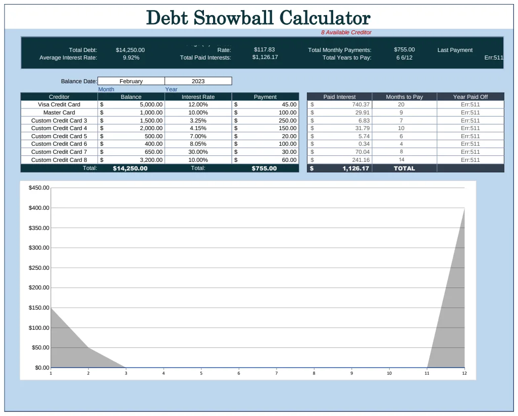
Build your debt snowball spreadsheet in Google Sheets fast by focusing on clear data entry and a simple, accurate structure.
The most common reason a debt snowball spreadsheet in Google Sheets fails is a lack of clear, actionable data entry. People often get bogged down in how to set it up, rather than focusing on consistently inputting their actual payment amounts and dates. This leads to a spreadsheet that looks pretty but doesn't reflect reality, defeating the purpose of a debt snowball spreadsheet Google Sheets template.
To build a functional debt snowball spreadsheet in Google Sheets, you need a clear structure that prioritizes simplicity and accuracy. The core idea of the snowball method is to pay off your smallest debts first while making minimum payments on the others. Once a debt is paid off, you roll that payment amount into the next smallest debt, creating a "snowball" effect. A well-designed Google Sheets template can automate much of this, but it relies on you feeding it the right information.
Setting Up Your Debt Snowball Tracker
Start by creating a new Google Sheet. You'll need several columns to track your progress effectively. Aim for clarity over complexity.
Here’s a suggested setup for your main tracking sheet:
- Debt Name: The name of the creditor (e.g., "Visa Card," "Student Loan," "Car Payment").
- Starting Balance: The total amount owed on that debt when you begin.
- Minimum Payment: The required monthly payment from your lender.
- Interest Rate (%): The Annual Percentage Rate (APR) for that debt. This is crucial for understanding how much interest you're paying.
- Payoff Order (Snowball): A simple number indicating the order in which you'll tackle the debts, from smallest balance to largest.
- Extra Payment: Any additional amount you plan to pay on this debt each month beyond the minimum. This is the engine of your snowball.
- Total Monthly Payment: This column will sum the minimum payment and the extra payment for this specific debt.
- Current Balance: This will dynamically update as you make payments. You’ll need a formula here.
- Next Payment Due Date: Helps you stay on track with when payments are due.
- Status: A simple indicator like "Active," "Paid Off," or "On Hold."
You can create a separate sheet for a detailed payment log, which is where you'll record each actual payment made. This log will include columns like:
- Date Paid: When the payment was actually sent.
- Debt Name: Which debt the payment was for.
- Amount Paid: The total amount of the payment.
- Applied to Principal: How much of that payment went towards reducing the balance after interest.
- Interest Paid: How much of that payment covered interest charges.
Automating Calculations with Formulas
Google Sheets becomes powerful when you let formulas do the heavy lifting. For your main tracking sheet, you'll want a few key formulas.
In the Total Monthly Payment column (let’s assume this is column G), your formula would be: =SUM(F2,C2) This simply adds your extra payment (column F) to the minimum payment (column C) for that specific debt, assuming row 2.
The Current Balance column (column H) is where things get interesting. This will require a formula that references your payment log. A common approach is to use SUMIFS to sum up all payments made to a specific debt and subtract that from the starting balance. However, this can get complicated quickly if you're trying to account for interest accrual within the same sheet.
A more robust solution is to have your payment log calculate interest and principal applied, and then your main sheet simply subtracts the "Applied to Principal" from the starting balance. For a simpler version, you could use a formula like: =C2 - SUMIFS('Payment Log'!$D:$D, 'Payment Log'!$B:$B, A2) This formula, placed in H2, assumes your "Payment Log" sheet has payments recorded in column D, the debt name in column B, and you're matching the debt name in your main sheet's column A. This formula only accounts for principal payments and doesn't dynamically add interest, so it's a simplified view. For more accuracy, consider a dedicated debt payoff calculator template.
Implementing the Snowball Logic
The "Payoff Order" column is critical. You'll manually assign these numbers (1, 2, 3, etc.) based on the smallest starting balance to largest. Your strategy is to put all available extra payment money towards the debt marked "1." Once that debt's balance reaches zero, you then add its minimum payment and its extra payment to the minimum payment of the debt marked "2."
This requires a bit of manual adjustment or a more complex setup. You might have a separate "Summary" tab. On this summary tab, you could have a formula like: =MIN(C2:C10) + IF(H2=0, MAX(F2:F10), 0) This is a highly simplified example. A real-world scenario often involves a control panel where you input your total available debt payment amount. Then, formulas dynamically allocate the minimum payments to all debts and the remaining extra amount to the debt currently in the "Payoff Order" number 1. Once that debt is paid off (its current balance hits zero), the formula shifts the extra amount to the next debt in line.
For a more automated approach that handles this dynamic allocation, you might find a dedicated template helpful. Tools like the Debt Reduction Calculator can help you visualize this snowball effect more clearly.
Tracking Progress Visually
Humans are visual creatures. Seeing your progress can be a powerful motivator. Google Sheets offers several ways to visualize your debt snowball efforts.
- 01Progress Bars: You can use conditional formatting to create visual progress bars in your "Current Balance" column. Select the "Current Balance" column (H), go to "Format" > "Conditional formatting." Choose "Color scale." Set the minimum value to 0 and the maximum value to your "Starting Balance" (column B). Choose a color scale that shows progress from red (high balance) to green (paid off).
- 02Charts: Create a bar chart or line chart to show how your total debt is decreasing over time. You can plot "Date Paid" against the "Total Debt Remaining" (a column you'd sum up from your current balances). Another useful chart is one that shows the debt allocation, how much is going to minimum payments versus extra payments.
- 03Summary Dashboard: A separate sheet can serve as a dashboard. It could display:
- Total Debt Remaining
- Total Paid This Month
- Number of Debts Paid Off
- Projected Payoff Date (this requires more advanced formulas, possibly involving iterative calculations if you want to be precise about interest)
A well-designed visual dashboard can make managing your debt snowball spreadsheet Google Sheets template much more engaging.
Common Pitfalls to Avoid
Even with a great template, you can stumble. Here are a few common mistakes:
- Inconsistent Data Entry: This is the biggest killer. If you don't log payments regularly and accurately, your spreadsheet becomes useless.
- Not Updating Interest Rates: If your interest rates change, or if you started with inaccurate ones, your payoff projections will be off.
- Ignoring Fees: Some debts might have annual fees or late fees that can derail your plan if not accounted for.
- Adding New Debt: The snowball method works best when you're not taking on new debt. If you must, adjust your plan immediately.
- Overly Complex Formulas: While automation is great, don't build a system so complicated that you can't understand or fix it. Start simple and add complexity only if needed.
- Not Factoring in Extra Payments: The "extra payment" is the key. If you don't consistently apply extra money, the snowball won't build momentum.
If you find yourself struggling to build this complexity from scratch, exploring a pre-built solution can save time. The Debt Snowball Excel Spreadsheet offers a comprehensive system, and its principles can be adapted to Google Sheets.
Advanced Tips and Customization
Once you have the basics down, you can enhance your debt snowball spreadsheet Google Sheets setup.
- Conditional Formatting for Due Dates: Set up rules to highlight upcoming or past-due payments. For instance, if "Next Payment Due Date" (column I) is within the next 7 days, turn the cell yellow. If it's past due, turn it red.
- Calculating Interest vs. Principal: For a more accurate picture, consider adding columns to your "Payment Log" that attempt to estimate how much of each payment goes to interest and how much to principal. This is complex because interest accrues daily, but a monthly approximation can be useful. Many online calculators provide this breakdown.
- Scenario Planning: Use your spreadsheet to test different scenarios. What if you could find an extra $50 per month? How much faster would you be debt-free?
Remember, the goal is to create a tool that motivates you and provides clarity. A debt snowball spreadsheet Google Sheets template should simplify your financial life, not complicate it.
What if my interest rates change?
If your interest rates change (e.g., a variable rate loan or a promotional period ending), you'll need to update the "Interest Rate (%)" column for that specific debt. This will affect your projected payoff timeline and the total interest paid. For a dynamic adjustment, you might need to rebuild the formulas that calculate interest accrual or, more simply, use a tool that allows for easy rate updates. The Credit Repair Calculator can help visualize different payoff strategies with varying interest rates.
How do I handle multiple minimum payments and then add extra?
This is the core of the snowball. Once you've identified your smallest debt (based on balance), you make its minimum payment, plus any extra payment you've allocated. For all other debts, you make only their minimum payments. When the smallest debt is paid off, you take its minimum payment and add it to the extra payment for the next smallest debt. This requires you to manually adjust your payment allocations each time a debt is cleared, or to build a more sophisticated system that automatically reallocates funds based on debt status.
Can I use this for more than just credit cards?
Absolutely. The debt snowball method can be applied to any type of debt: personal loans, student loans, car payments, and even mortgages if you're aggressive about paying them down. The key is to list all your debts, order them by balance, and consistently apply the snowball strategy. You might find that different debt types have different payment structures or rules, so ensure your spreadsheet accommodates these variations in the "Minimum Payment" and "Interest Rate" columns.