Where can I find a free Excel savings tracker template?
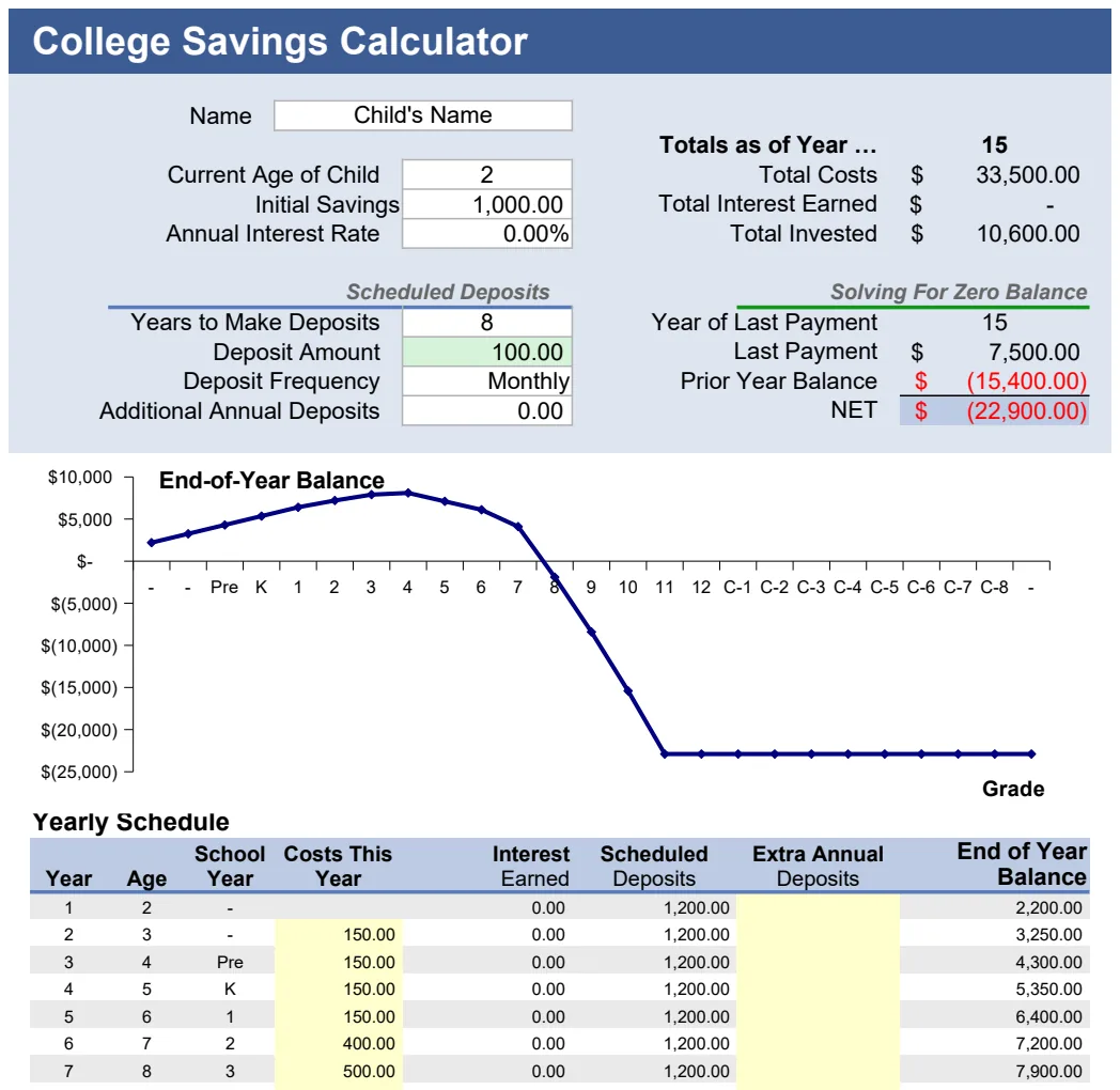
Find a free savings tracker template in Excel to easily log transactions and see your progress at a glance.
Using a spreadsheet for savings is usually better than a notebook, but a well-built savings tracker template Excel free can save you hours of setup. Many free templates exist, but most are either too basic to be useful or overly complicated with features you’ll never touch. You need a straightforward system that lets you log transactions and see your progress at a glance.
A good savings tracker focuses on clarity and automation. It should automatically sum your deposits and withdrawals, update your running balance, and clearly show how much closer you are to your goals. Think of it as a digital ledger that does the math for you.
Why a Template Beats a Blank Sheet
Starting from scratch with a blank Excel sheet means defining every column, writing every formula, and setting up all the formatting yourself. For a basic tracker, that might take an hour or two. For something more robust, it could take much longer. A pre-built template, like the Savings Goal Tracker, gives you a solid foundation. You can start logging your savings within minutes, focusing on your goals rather than spreadsheet mechanics. This is especially true if you're looking for a savings tracker template Excel free that’s both functional and easy to adapt.
Consider this: if you're aiming to save $10,000 for a down payment, and you're starting with $500, you need to track your progress. Manually calculating your remaining balance after each deposit or withdrawal would be tedious. A template handles this automatically. It’s the difference between meticulously adding up numbers in a notebook and having a dashboard that updates in real-time. You're paying for convenience and accuracy, even when the template itself is free.
Furthermore, a template often comes with pre-configured conditional formatting. For example, it might highlight deposits in green and withdrawals in red, or visually indicate when you're falling behind on a savings target. This visual feedback is incredibly powerful for motivation. Without a template, you'd have to know how to set up these rules yourself, which involves understanding Excel's conditional formatting options and writing the correct logic.
Essential Components of a Savings Tracker
No matter which template you choose, look for these core elements:
- Transaction Log: A clear table to record every deposit and withdrawal. This is the heart of your tracker.
- Date: When the transaction occurred. Accurate dates are vital for chronological tracking and analysis.
- Description: What the transaction was for (e.g., "Paycheck Deposit," "Rent Payment," "Transfer to Savings," "ATM Withdrawal"). Specificity here helps you understand your spending habits.
- Category: Optional, but highly recommended. This allows you to group transactions (e.g., "Income," "Bills," "Savings Transfer," "Fun Money"). This is key for understanding where your money is going beyond just deposits and withdrawals.
- Type: Whether it's a "Deposit" or "Withdrawal." This is crucial for calculations. A simple dropdown list is best.
- Amount: The value of the transaction. This should be a numerical field.
- Running Balance: This is arguably the most important part. It shows your total savings after each transaction. This field needs to update automatically.
Beyond these basics, advanced trackers might include dedicated sections for specific savings goals (like "Emergency Fund," "Vacation Fund," "New Car"), each with its own target amount and progress bar. They might also offer automatic calculations for projected balances based on your average savings rate, or even integrate with other financial tracking tools if you're using a more complex system.
Setting Up Your Transaction Log
Let's walk through setting up a simple transaction log. Imagine you have a sheet named "Transactions."
Columns:
- A: Date: Format this column as a Date. This ensures Excel recognizes it as such, enabling sorting and filtering by date.
- B: Description: This is a text field. Keep it concise but informative.
- C: Category: Create a dropdown list for this column. Go to "Data" > "Data Validation." Select "List" and in the "Source" box, enter your categories separated by commas, like:
Income, Bills, Savings Transfer, Expenses, Miscellaneous. This enforces consistency. - D: Type: Another dropdown list. Select "Deposit" and "Withdrawal." This is critical for formulas.
- E: Amount: This column should be formatted as a Number or Currency.
- F: Running Balance: This is where the magic happens.
Formulas for the Running Balance:
For the first transaction (let's assume it's in row 2): In cell F2, you'll enter a formula that checks the "Type" and adds or subtracts the "Amount" from your starting balance. If you have an initial balance in cell G1 (e.g., $1000), the formula in F2 would be:
=G1 + IF(D2="Deposit", E2, -E2)
This formula says: "Take the starting balance (G1), and if the 'Type' in D2 is 'Deposit', add the 'Amount' from E2. Otherwise (if it's a 'Withdrawal'), subtract the 'Amount' from E2."
For all subsequent rows (from row 3 downwards): In cell F3, the formula needs to reference the previous running balance. So, the formula becomes:
=F2 + IF(D3="Deposit", E3, -E3)
You can then drag this formula down from F3 to the last row of your transactions. Excel will automatically adjust the cell references (F2 will become F3, D3 will become D4, and E3 will become E4, and so on).
Example Data:
| Date | Description | Category | Type | Amount | Running Balance | | :--------- | :---------------- | :------------- | :------- | :----- | :-------------- | | 2026-01-01 | Initial Deposit | Income | Deposit | 1000 | 1000.00 | | 2026-01-05 | Paycheck | Income | Deposit | 1500 | 2500.00 | | 2026-01-10 | Rent Payment | Bills | Withdrawal | 800 | 1700.00 | | 2026-01-12 | Transfer to Savings | Savings Transfer | Deposit | 500 | 2200.00 | | 2026-01-15 | Groceries | Expenses | Withdrawal | 150 | 2050.00 |
Notice how each "Running Balance" in column F is calculated based on the previous row's balance and the current transaction's type and amount.
Tracking Progress Towards Goals
A savings tracker isn't just about logging transactions; it's about seeing how far you've come and how far you have to go.
Dedicated Goal Section:
If you're using a template with goal tracking, you'll typically find a separate area, perhaps on a dashboard sheet or at the top of your transaction log. This section might have columns like:
- Savings Goal: Name of the goal (e.g., "Emergency Fund").
- Target Amount: The total amount you need to save.
- Amount Saved: This formula needs to sum up all deposits specifically allocated to this goal. If you use a "Category" column in your transaction log and label goal-related deposits as "Emergency Fund Deposit," you could use a
SUMIFformula. For example, if your transactions are in Sheet1 and your goal is on Sheet2 in cellB2(target amount), and you want to calculate the amount saved for this goal, the formula inC2of Sheet2 might look like this:
=SUMIF(Sheet1!D:D, "Emergency Fund Deposit", Sheet1!E:E)
This formula sums amounts in Sheet1's column E (Amount) where the corresponding cell in Sheet1's column D (Category) is exactly "Emergency Fund Deposit."
- Remaining Amount: A simple subtraction:
Target Amount-Amount Saved. - Progress %:
(Amount Saved / Target Amount) * 100. Format this column as a Percentage. - Visual Indicator: Many templates use conditional formatting here. For example, a data bar within the cell that fills up as the "Amount Saved" increases, or the cell color changing from red to green as you get closer to the target.
Example Goal Tracking:
Let's say you have two goals: "Emergency Fund" ($5,000 target) and "Vacation Fund" ($2,000 target).
| Savings Goal | Target Amount | Amount Saved | Remaining Amount | Progress % | | :---------------- | :------------ | :----------- | :--------------- | :--------- | | Emergency Fund | 5000 | 2200 | 2800 | 44.00% | | Vacation Fund | 2000 | 500 | 1500 | 25.00% |
The "Amount Saved" figures would be dynamically calculated from your transaction log, and the "Progress %" would update automatically.
Automating Your Savings Calculations
The real power of a spreadsheet template lies in its ability to automate calculations, saving you time and reducing errors.
Summing Deposits and Withdrawals:
Beyond the running balance, you might want to see your total income and total expenses for a given period.
- Total Deposits: Use the
SUMIFfunction. If your "Type" column is D and "Amount" is E, and you want to sum all "Deposit" entries:
=SUMIF(D:D, "Deposit", E:E)
- Total Withdrawals: Similarly:
=SUMIF(D:D, "Withdrawal", E:E)
Calculating Net Savings: This is simply your total deposits minus your total withdrawals. If your total deposits sum to cell G10 and total withdrawals to G11, the net savings would be =G10-G11.
Projecting Future Balances: A more advanced feature might project your balance into the future. This requires calculating your average net savings per period (e.g., per week or month).
- 01Calculate Net Savings per Period: You'd need to sum deposits and withdrawals for specific date ranges. Using
SUMIFSis ideal here. For example, to get net savings for January:
=SUMIFS(E:E, D:D, "Deposit", A:A, ">=2026-01-01", A:A, "<=2026-01-31") - SUMIFS(E:E, D:D, "Withdrawal", A:A, ">=2026-01-01", A:A, "<=2026-01-31") (Assuming Date is column A, Type is D, Amount is E).
- 02Calculate Average Net Savings: Once you have net savings for several periods, you can average them. If your monthly net savings are in cells
H2(Jan),H3(Feb), etc., you can average them with=AVERAGE(H2:H13).
- 03Project Future Balance: Take your current balance (the last value in your running balance column) and add your average net savings multiplied by the number of future periods. For example, to project one month ahead:
=LastRunningBalance + AverageMonthlyNetSavings
This level of automation turns your spreadsheet from a simple ledger into a powerful financial planning tool.
Common Mistakes to Avoid
Even with a good template, users can make mistakes that undermine the accuracy of their savings tracking.
- Inconsistent Data Entry: Failing to categorize transactions consistently, or misspelling category names, will break
SUMIFandSUMIFSformulas. Always use dropdowns where possible and stick to the exact wording. - Ignoring Small Transactions: It's tempting to overlook a small cash withdrawal or a minor deposit, but these add up. Diligent logging is key.
- Not Updating Regularly: If you let transactions pile up, it becomes a daunting task to enter them all later, increasing the chance of errors or omissions. Aim to update your tracker daily or at least weekly.
- Mixing Personal and Business Finances: If you use a template for personal savings, don't mix in business income or expenses. This will skew your personal savings calculations. Use separate trackers or sheets for different financial contexts.
- Incorrect Formulas: Double-check your running balance formula, especially the initial setup and how it references the previous row. A single error here can cascade and make your entire balance incorrect. Ensure you're using
IF(D2="Deposit", E2, -E2)or a similar logic, not just=F2+E2. - Forgetting the Starting Balance: If you have money in savings before you start using the template, make sure that initial amount is logged as the very first transaction (a deposit).
Customizing Your Savings Tracker Template
While free templates offer a great starting point, you'll likely want to tailor them to your specific needs.
Adding More Specific Goals: If your template has a section for just three goals and you have five, you can usually duplicate the rows for the goal section and adjust the formulas. Ensure the new SUMIF formulas correctly reference the new categories you'll need to add to your transaction log's dropdown list. For example, if you add a "New Laptop" goal, you'll need to add "Laptop Deposit" to your transaction categories and update the SUMIF formula in the goal section to include this new category.
Changing Time Periods: Perhaps you want to track weekly savings instead of monthly. You might need to add a "Week Number" column to your transaction log (using the =WEEKNUM(A2) formula, assuming Date is in A2) and then adjust your SUMIFS formulas to sum based on week number in addition to date ranges.
Visual Enhancements: You can add charts to visualize your savings growth over time. Select your date column and your running balance column, then go to "Insert" > "Chart." A line chart is usually best for showing trends. You can also add pie charts to show the breakdown of your savings categories or expenses.
Adjusting the Running Balance Formula for Different Starting Points
What if your initial deposit isn't the very first entry? Or what if you're starting mid-month?
The key is that the first cell in your running balance column must correctly reflect the balance after the first transaction. If your starting balance from an existing account is $5,000 and your first transaction logged is a $100 deposit on January 10th, the formula for that first row (let's say row 5) would be:
=5000 + IF(D5="Deposit", E5, -E5)
For all subsequent rows (row 6 onwards), the formula remains the same structure, referencing the previous row's balance:
=F5 + IF(D6="Deposit", E6, -E6)
This ensures that the initial lump sum is accounted for before the transaction-by-transaction calculation begins.
Integrating Savings Goals with the Overall Balance
It's common to have a general savings pool and also specific pots for goals. How do you reconcile this?
Your main "Running Balance" column should reflect your total available cash. If you transfer money from your main account to a specific "Vacation Fund" savings account, this should be logged as a withdrawal from your main account and a deposit into the "Vacation Fund" tracker.
The "Amount Saved" for each goal should sum deposits specifically designated for that goal. If you have a transaction like "Transfer to Vacation Fund" in your main transaction log, and you've categorized it as "Savings Transfer," your goal tracker's SUMIF formula would look for that specific category to add to the "Vacation Fund" total. The total of all "Amount Saved" across all your goals should ideally not exceed your total "Amount Saved" in your main tracker. This prevents you from over-allocating money you don't actually have.
Handling Irregular Income or Expenses
Life isn't always predictable. If your income or expenses fluctuate wildly, your average savings rate projection might be inaccurate.
In such cases, rely more on the "Running Balance" and less on projections. Focus on ensuring each deposit and withdrawal is accurately logged. For goal tracking, the SUMIF approach is still robust because it sums actual contributions, regardless of when they occurred. If you have a month with very low savings due to an unexpected expense, your goal progress might slow, but the tracker will accurately reflect that. You can always adjust your goal timelines if needed, based on the actual progress shown.